|
Description of Meteorological Conditions During an Episodic Surface Ozone Event
Samuel J. Oltmans, Climate Monitoring and Diagnostics Laboratory, NOAA, Boulder, CO Allen S. Lefohn, A.S.L. & Associates, Helena, MT November 7, 2001
The high surface ozone concentrations observed at the Haywood County, NC site (AIRS ID 370870035) in western North Carolina from April 28 through May 1, 2000, culminating in the hourly average ozone reading of 93 ppb late in the day on May 1 (LST), appear to be a case of a dry airstream influenced by a stratospheric intrusion reaching the surface (see Lefohn et al., 2001 and Cooper et al., 2001 for a description of this type of system). Figure 1 shows the hourly average concentrations for the period April 26 - May 3, 2000. Both trajectory analysis (Figures 2 and 3) and an examination of water vapor imagery (Figure 4) from the GOES operational weather satellite provide evidence that dry air from the backside of an upper air trough was streaming down from higher altitudes over Canada. Isentropic trajectories at 1.7 km beginning on April 28 show air streaming southward from Hudson Bay throughout the period reaching western North Carolina within 5 days. A deep trough was located in northeastern Canada and a strong pressure ridge dominates the central portion of the U.S. at 500 hPa (~ 5.5 km). This blocking pattern persists through the period thus promoting the flow from the north on the leading edge of the ridge (back side of the trough). For the trajectory late on May 1, there had been particularly strong descent of air parcels beginning five days earlier over Canada. It appears likely that air mixed into the troposphere from the stratosphere, possibly in a tropopause-folding event over Canada, contributed significantly to the high ozone measured over North Carolina. The May 1 episode resulted in the second highest 8-hour value during 2000 and this meant that the 4th highest was 0.085 ppm for the year. If this event were eliminated, the 4th highest 8-hour daily maximum concentration would have been 0.082 ppm.
ReferencesCooper, O.R., J.L. Moody, D.D. Parrish, M. Trainer, T.B Ryerson, J.W. Holloway, G. Hüber, F.C. Fehsenfeld, S.J. Oltmans, and M.J. Evans. 2001. Trace gas signatures of the airstreams within North Atlantic cyclones: Case studies from the North Atlantic Regional Experiment (NARE ’97) aircraft intensive. J. Geophys. Res. 106(D6):5437-5456.
Lefohn, A.S., S.J. Oltmans, T. Dann, and H.B. Singh. 2001. Present-day variability of background ozone in the lower troposphere. J. Geophys. Res. 106(D9):9945-9958. |
Height of the 500 hPa Surface
April 30 - May 1, 2000
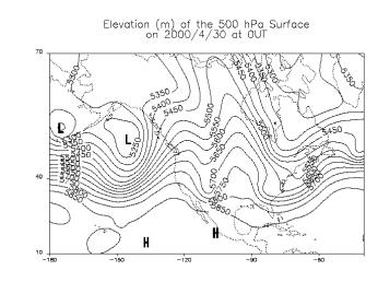
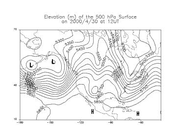
Figure 2a Figure 2b
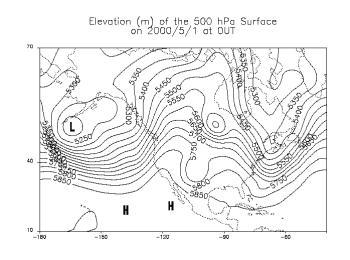
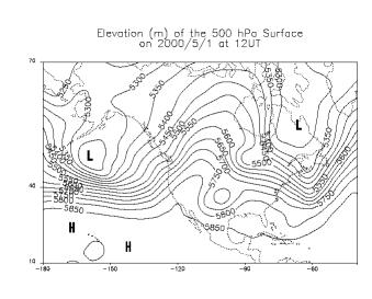
Figure 2c Figure 2d
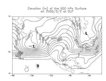
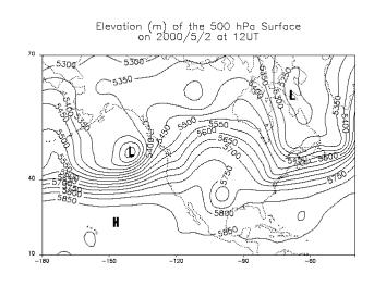
Figure 2e Figure 2f
Trajectories to Haywood County, NC (370870035) Ozone Site
April 28 - May 3, 2000
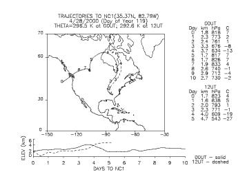
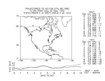
Figure 3a Figure 3b
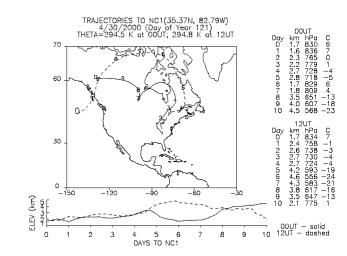
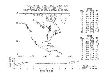
Figure 3c Figure 3d
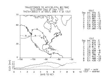
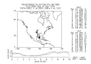
Figure 3e Figure 3f
Remotely sensed relative humidity in the middle and upper troposphere from the
Geostationary Operational Environmental Satellite (GOES) infrared water vapor channel.
Blue colors represent drier air; yellow and red colors moister air.
April 27 - May 2, 2000
Figure 4a. April 27, 2000 0600 UTC Figure 4b. April 27,
2000 1200 UTC
Figure 4c. April 27, 2000 1800 UTC Figure 4d. April 28,
2000 0000UTC
Figure 4e. April 28, 2000 0600 UTC Figure 4f. April 28,
2000 1200 UTC
Figure 4g. April 28, 2000 1800 UTC Figure 4h. April 29,
2000 0000 UTC
Figure 4i. April 29, 2000 0600 UTC Figure 4j. April 29,
2000 1200 UTC
Figure 4m. April 30, 2000 0600 UTC Figure 4n. April 30, 2000
1200 UTC
Figure 4o. April 30, 2000 1800 UTC Figure 4p. May 1,
2000 0000 UTC
Figure 4s. May 1, 2000 1800 UTC Figure 4t. May 2,
2000 0000 UTC