Introduction
Lefohn et al. (2008) summarized their trends
analyses for surface ozone monitoring sites across the United
States. Using statistical trending on a site-by-site basis of
the (1) health-based annual 2nd highest 1-hour average concentration
and annual 4th highest daily maximum 8-hour average concentration
and (2) vegetation-based annual seasonally corrected 24-hour
W126 cumulative exposure index, they investigated temporal and
spatial statistically significant changes that occurred in surface
ozone in the United States for the periods 1980-2005 and 1990-2005
and explored whether differences in trending occur depending
upon the selection of the exposure metric. Using the trending
results, the analyses quantitatively explore the evidence for
the higher hourly average ozone concentrations decreasing faster
than the mid- and lower-values.
Results
Figure 1 below from Lefohn et al. (2008) summarizes
the findings for the trending of the 4th highest 8-hour ozone
metric for the 1980-2005 and 1990-2005 periods.
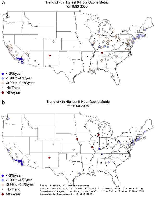
Figure 1. Trend of 4th highest 8-hour average
ozone metric for the (a) 1980-2005 and (b) 1990-2005 periods.
This figure was published in Lefohn et. al. (2008). Copyright
Elsevier. Please see reference below. Permission granted by Elsevier
to reproduce the above figure only on this web page.
Most of the surface ozone monitoring sites
analyzed in the study experienced decreasing or no trends. Few
monitoring sites experienced increasing trends. For those monitoring
sites with declining ozone levels, an initial pattern of rapid
decrease in the higher hourly average concentrations, followed
by a much slower decrease in mid-level concentrations was observed.
In some cases, they observed shifts from the lower hourly average
ozone concentrations to the mid-level values. On a site-by-site
basis, the majority of monitoring sites (1) changed from negative
trend to no trend, (2) continued a negative trend, or (3) remained
in the no trend status, when comparing trends for the 1980-2005
to the 1990-2005 time periods. For the three exposure metrics
(i.e., annual 2nd highest 1-hour average concentration, annual
4th highest daily maximum 8-hour average concentration, and vegetation-based
annual seasonally corrected 24-hour W126 cumulative exposure
index, approximately 60% of the monitoring sites shifted from
negative trending to no trending status. All regions of the United
States were equally affected by the shift in status.
Lefohn et al. (2008) in their paper provide
several figures that illustrate the spatial patterns of trends
across the United States. The greatest statistically significant
decreases in the 2nd highest 1-hour average concentrations and
the annual 4th highest daily maximum 8-hour average concentration
for the two temporal periods occurred in southern California.
Monitoring sites in other portions of the United States experienced
lesser decreases than this geographic area. In contrast to the
two exposure indices, the vegetation-based 24-hour W126 ozone
cumulative index for 1980-2005 experienced significant declines
in the midwestern states and the northeastern United States,
as well as in southern California. For the 1990-2005 period,
monitoring sites in southern California and the northeastern
United States experienced the greatest decreases in the W126
exposure metric.
When trending was observed, not all months
experienced trending. Lefohn et al. (2008) tested for statistically
significant changes in the number of hourly average concentrations
within specified concentration intervals and identified specific
months that experienced shifts in the distribution of the hourly
average concentrations. As an example, Figures 2 and 3 below
illustrate the changes in the distribution of the hourly average
ozone concentrations for a monitoring site located in Reseda
in Los Angeles County as reductions occurred over the 1980-2005
and 1990-2005 periods.
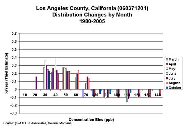
Figure 2. Distribution of changes by month
for a monitoring site located in Los Angeles County, California
(AQS 060371201) for 1980-2005 for the months with significant
changes.
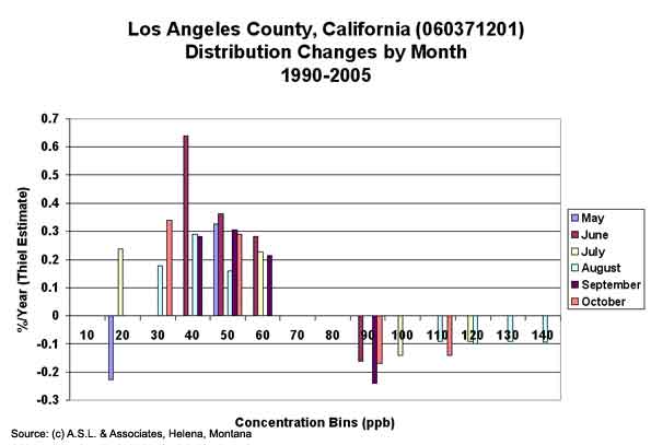
Figure 3. Distribution of changes by month
for a monitoring site located in Los Angeles County, California
(AQS 060371201) for 1990-2005 for the months with significant
changes.
The two figures show the reductions in the
number of hourly average concentrations in the higher hourly
average concentrations and the increases in the mid-level concentrations
as the peak values were reduced.
The Theil estimate was used to estimate trending.
The Theil estimate is determined as the median of slope estimates
calculated as the slope of the line passing through two points
for all pairs of points in the data set of interest. To test
for statistical significance, Kendall's tau test was used to
determine significance at the 10% level.
The Mann-Kendall (M-K) nonparametric test
is utilized to test for a significant trend. Advantages of the
M-K test are
- No distributional assumption is made;
- No assumption of any specific functional
form for the behavior of the data through time is made. Thus,
the M-K test is universally applicable across all sites, seasons,
and different continuous summary exposure metrics (e.g., percentiles,
means, and cumulative exposure indices, such as the W126 and
AOT40 vegetation exposure metrics); and
- The M-K test is resistant to the effects
of outlying observations. The results are not unduly affected
by particularly high or low values that occur during time series
analyses.
For estimating the magnitude of a trend, the
Theil-Sen (also called Sen-Theil, Theil, or Sen) estimator can
be used. It possesses the same attributes described above for
the M-K test (i.e., there are no distributional or functional
form assumptions and the estimator is resistant to outliers).
The Theil-Sen (T-S) estimator, similar to the M-K technique,
is also universally applicable. In cases where simple linear
regression is appropriate (assuming key assumptions are met),
the slope of the regression line and the T-S estimator are asymptotically
equivalent.
For more information about the Theil estmate
and the Kendall's tau test, please see the discussion in Section
3 in Lefohn et al. (2018).
Note that the months of March and April exhibited
statistically significant trending in the 1980-2005 period, but
did not exhibit statistically significant trending over the 1990-2005
period. Over the 1990-2005 period, the month of September exhibited
statistically significant trending but did not over the 1980-2005
period.
Lefohn et al. (2010a) updated the trending
results reported in Lefohn et al. (2008). The updated trending
periods were 1980-2008 (29 years) and 1994-2008 (15 years). In
addition to updating the trends analysis, the authors focused
on 12 urban and 15 rural monitoring sites. The trending results
provide examples on why it is important
to investigate the change in the trending pattern with time (e.g.,
moving 15-year trending) in order to assess how year-to-year
variability may influence the trend calculation. Several research
investigations have explored trending from the beginning of a
data series until the latest date for collection of data. However,
these types of trends analyses do not take into consideration
the possibility that the rate of trending over the period of
record has changed and in some cases the trending has ceased.
Lefohn et al. (2010a) took a closer look at changes in the rate
of trending and drew conclusions about the importance of using
15-year moving trends to quantify trending rates. The paper's
abstract is available on our publications web page.
Conclusions and Recommendations
Most of the surface ozone monitoring sites
analyzed in the Lefohn et al. (2008, 2010a) studies experienced
decreasing or no trends. Few monitoring sites experienced increasing
trends. Lefohn et al. (2008, 2010a) observed that a statistically
significant trend at a specific monitoring site, using one exposure
index, did not necessarily result in a similar trend using the
other two indices. The authors recommended that because different
trending patterns were observed when applying the various exposure
indices, a careful selection of ozone exposure metrics is required
when assessing trends for specific purposes, such as human health,
vegetation, and climate change effects. Lefohn et al. (2017)
performed a detailed analysis using several human health and
vegetation exposure metrics and quantified the differences in
trends using different metrics for sites in the US, EU, and China.
As in previous analyses, Lefohn et al. (2017) noted that using
the identical hourly average ozone concentrations, different
trend patterns occurred based on the selection of the specific
exposure indices (e.g., metrics focused on the higher end of
the distribution versus those indices focused on the lower end
of the distribution). In some cases, the high end of the distribution
moved downward, while the low end of the distribution shifted
upward. The lower hourly averaged ozone concentrations moved
upward due to less titration of ozone by NO as reduction in NOx
emissions occurred (Lefohn et al., 1998; Lefohn et al., 2010a;
Tørseth et al., 2012; Simon et al., 2015; Lefohn et al.,
2017, 2018; Aas et al., 2024; Real et al., 2024). For
assessing biological effects, the highest hourly average ozone
concentrations are more important than the mid- and low-level
values for human health (Hazucha and Lefohn, 2007; Lefohn et
al., 2010b) and vegetation (Musselman et al., 2006; Hogsett et
al., 1985; Lefohn et al., 2018).
Part 2 - Ozone
Trends of Special Monitoring Stations for Assessing Background
Ozone Trending
Introduction
Over the past several years,
there have been several articles quoting other sources indicating
that surface ozone concentrations are increasing everywhere.
Our research results do not support this claim. Our research
efforts monitor the status of worldwide ozone levels by performing
sophisticated analyses using surface ozone and ozonesonde data
(e.g., Oltmans et al., 1998; Oltmans et al., 2006; Oltmans et
al., 2013). Our research focuses on the results from the available
data from four decades of observations for the longest records
(ozonesondes). Several key stations have 30-40 years of observations
for both surface and ozonesondes. The key ozone monitoring stations
provide good data for the purpose of assessing possible changes
in background levels of ozone. Some of the sites offer the opportunity
to study records representative of broad geographic regions where
local effects are minimized.
Oltmans et al. (2013) discusses the longer-term (i.e., 20-40 years) tropospheric
ozone time series obtained from surface and ozonesonde observations
that we analyzed to assess possible changes with time through
2010. The time series have been selected to reflect relatively
broad geographic regions and where possible minimize local scale
influences, generally avoiding sites close to larger urban areas.
Several approaches have been used to describe the changes with
time, including application of a time-series model, running 15-year
trends, and changes in the distribution by month in the ozone
mixing ratio. Changes have been investigated utilizing monthly
averages, as well as exposure metrics that focus on specific
parts of the distribution of hourly average concentrations (e.g.,
low-, mid-, and high-level concentration ranges). Oltmans et
al. (2013) noted that many of the longer time series (~30 years)
in mid-latitudes of the Northern Hemisphere, including those
in Japan, show a pattern of significant increase in the earlier
portion of the record, with a flattening over the last 10-15
years. It is uncertain if the flattening of the ozone change
over Japan reflects the impact of ozone transported from continental
East Asia in light of reported ozone increases in China. In the
Canadian Arctic, declines from the beginning of the ozonesonde
record in 1980 have mostly rebounded with little overall change
over the period of record. The limited data in the tropical Pacific
suggest very little change over the entire record. In the southern
hemisphere subtropics and midlatitudes, the significant increase
observed in the early part of the record has leveled off in the
most recent decade. At the South Pole, a decline observed during
the first half of the 35-year record has reversed, and ozone
has recovered to levels similar to the beginning of the record.
Our understanding of the causes of the longer-term changes is
limited, although it appears that in the mid-latitudes of the
Northern Hemisphere, controls on ozone precursors have likely
been a factor in the leveling off or decline from earlier ozone
increases.
As indicated earlier in the
Part 1 discussion, it is important to investigate the rate-of-change
in trending and not just analyze for trends using the beginning
and ending periods of monitoring. For example, Logan et al. (2012)
described the decrease in ozone over Europe since 1998, with
the largest decrease during the summertime. Using Zugspitze data
for 1978-1989 and the mean time series from three Alpine stations
since 1990, Logan et al. (2012) found that the ozone increased
substantially in 1978-1989 (i.e., 6.5-10 ppb but began to exhibit
a reduced rate of increase in the 1990s (i.e., 2.5-4.5 ppb) with
decreases in the 2000s (i.e., 4 ppb) in summer with no significant
changes in other seasons. Overall in summer no trend was noted
for the 1990-2009 period.
Conclusions and Recommendations
Our results suggest
that on a hemispheric scale it is currently difficult to observe
the projected increases in tropospheric ozone that models indicate
may occur from Asian emissions. This may result from the lack
of such ozone increases or that changes resulting from precursor
reductions in North America and Europe have made the influence
of Asian precursor emissions more difficult to detect. Parrish
et al. (2017) noted that over the past decades, a long-term increase
in baseline ozone has been observed at the North American west
coast. They concluded, based on their analyses, this increase
has ended. These results complement our observation that changes
in hourly average ozone distributions at the low-, mid and high-level
ranges for sites investigated in our most recent study do not
indicate that background ozone concentrations continue to increase
in the most recent decades. As indicated in our analysis and
others, at many of the investigated sites earlier ozone increases
have reached a plateau and in some cases begun to decrease. In
order to follow future trend patterns, it will be important to
use techniques that capture the time evolution of ozone changes,
such as the 15-year trend periods used by Lefohn et al. (2010a)
and Oltmans et al. (2013) or other methods that detect these
changes. Due to the increase in the frequency of wildfires, it
will be important to identify changing trend patterns associated
with changing ozone precursors so as to better understand how
climate change is affecting current ozone levels.
References
Aas, W., Fagerli, H., Alastuey,
A., Cavalli, F., Degorska, A., Feigenspan, S., Brenna, H., Gliß,
J., Heinesen, D., Hueglin, C., Holubová, A., Jaffrezo,
J.L., Mortier, A., Murovec, M., Putaud, J.P., Rüdiger, J.,
Simpson, D., Solberg, S., Tsyro, S., Tørseth, K., Yttri,
K.E. (2024). Trends in Air Pollution in Europe, 2000-2019. Aerosol
Air Qual. Res. 24, 230237. https://doi.org/10.4209/aaqr.230237.
Hazucha, M. J.; Lefohn, A. S. (2007) Nonlinearity
in Human Health Response to Ozone: Experimental Laboratory Considerations.
Atmospheric Environment. 41:4559-4570.
Hogsett, W.E., Tingey, D.T., Holman, S.R.
(1985). A programmable exposure control system for determination
of the effects of pollutant exposure regimes on plant growth.
Atmos Environ 19: 1135-1145.
Lefohn A. S., Shadwick D.
S. and Ziman S. D. (1998). The Difficult Challenge of Attaining
EPA's New Ozone Standard. Environmental Science & Technology.
32(11):276A-282A.
Lefohn A. S., Shadwick D., and Oltmans S.
J. (2008). Characterizing long-term changes in surface ozone
levels in the United States (1980-2005). Atmospheric Environment.
42:8252-8262.
Lefohn, A. S., Shadwick, D.,
Oltmans, S. J. (2010a). Characterizing changes of surface ozone
levels in metropolitan and rural areas in the United States for
1980-2008 and 1994-2008. Atmospheric Environment. 44:5199-5210.
Lefohn, A.S., Hazucha, M.J.,
Shadwick, D., Adams, W.C. (2010b). An Alternative Form and Level
of the Human Health Ozone Standard. Inhalation Toxicology. 22
(12):999-1011.
Lefohn, A.S., Malley, C.S.,
Simon, H., Wells. B., Xu, X., Zhang, L., Wang, T., 2017. Responses
of human health and vegetation exposure metrics to changes in
ozone concentration distributions in the European Union, United
States, and China. Atmospheric Environment 152: 123-145. doi:10.1016/j.atmosenv.2016.12.025.
Lefohn, A.S., Malley, C.S.,
Smith, L., Wells, B., Hazucha, M., Simon, H., Naik, V., Mills,
G., Schultz, M.G., Paoletti, E., De Marco, A., Xu, X., Zhang,
L., Wang, T., Neufeld, H.S., Musselman, R.C., Tarasick, T., Brauer,
M., Feng, Z., Tang, T., Kobayashi, K., Sicard, P., Solberg, S.,
and Gerosa. G. (2018). Tropospheric ozone assessment report:
global ozone metrics for climate change, human health, and crop/ecosystem
research. Elem Sci Anth. 2018;6(1):28. DOI:
http://doi.org/10.1525/elementa.279.
Logan, J.A. et al. (2012).
Changes in ozone over Europe: Analysis of ozone measurements
from sondes, regular aircraft (MOZAIC) and alpine surface sites,
Journal of Geophysical Research, 117, D09031, doi:10.1029/2011JD16952.
Musselman R. C., Lefohn A.
S., Massman W. J., and Heath, R. L. (2006) A critical review
and analysis of the use of exposure- and flux-based ozone indices
for predicting vegetation effects. Atmospheric Environment. 40:1869-1888.
Oltmans S. J., Lefohn A. S.,
Scheel H. E., Harris J. M., Levy H. II, Galbally I. E. , Brunke
E. G., Meyer C. P., Lathrop J. A., Johnson B. J., Shadwick D.
S., Cuevas E., Schmidlin F. J., Tarasick D. W., Claude H., Kerr
J. B., Uchino O., and Mohnen V. (1998). Trends of ozone in the
troposphere. Geophysical Research Letters. 25:139-142.
Oltmans S. J., Lefohn A. S.,
Harris J. M., Galbally I., Scheel H. E., Bodeker G., Brunke E.,
Claude H., Tarasick D., Johnson B.J., Simmonds P., Shadwick D.,
Anlauf K., Hayden K., Schmidlin F., Fujimoto T., Akagi K., Meyer
C., Nichol S., Davies J., Redondas A., and Cuevas E. (2006).
Long-term changes in tropospheric ozone. Atmospheric Environment.
40:3156-3173.
Oltmans, S.J., Lefohn, A.S.,
Shadwick, D., Harris, J.M., Scheel, H.-E., Galbally, I., Tarasick,
D.A., Johnson, B.J., Brunke, E., Claude, H., Zeng, G., Nichol,
S., Schmidlin, F., Redondas, A., Cuevas, E., Nakano, T., Kawasato,
T. (2013). Recent Tropospheric Ozone Changes - A Pattern Dominated
by Slow or No Growth. Atmospheric Environment. 67:331-351.
Parrish D. D., Petropavlovskikh
I., Oltmans S. J. (2017). Reversal of long-term trend in baseline
ozone concentrations at the North American West Coast. Geophysical
Research Letters, 44, 10,675–10,681. https://doi.org/10.1002/2017GL074960.
Real, E., Couvidat, F., Chantreux, A., Megaritis,
A., Valastro, G., Colette, A. (2024). Assessing the Robustness
of Ozone Chemical Regimes to Chemistry-Transport Model Configurations.
Atmosphere. 15, 532. https://doi.org/10.3390/atmos15050532.
Simon H, Reff A, Wells B,
Xing J, Frank N. (2015). Ozone trends across the United States
over a period of decreasing NOx and VOC emissions. Environ Sci
Technol 49: 186-195. dx.doi.org/10.1021/es504514z.
Tørseth, K., Aas, W.,
Breivik, K., Fjæraa, A.M., Fiebig, M., Hjellbrekke, A.G.,
Lund Myhre, C., Solberg, S., and Yttri, K.E. (2012). Introduction
to the European Monitoring and Evaluation Programme (EMEP) and
observed atmospheric composition change during 1972–2009.
Atmos. Chem. Phys., 12, 5447–5481, 2012
www.atmos-chem-phys.net/12/5447/2012/doi:10.5194/acp-12-5447-2012.